Data is powerful—but only if it’s presented effectively. A well-designed chart can transform raw numbers into compelling insights, making it easier to identify trends, compare values, and tell a story.
Luckily, Microsoft Excel offers a wide range of charting and graphing tools that allow you to visualize data beautifully. Whether you’re working on financial reports, business analytics, or academic research, this guide will help you create stunning charts and graphs in Excel. 🚀
1️⃣ Choosing the Right Chart Type
Not all charts are created equal! Choosing the right type of chart depends on the kind of data you have and the story you want to tell. Here are some popular chart types and when to use them:
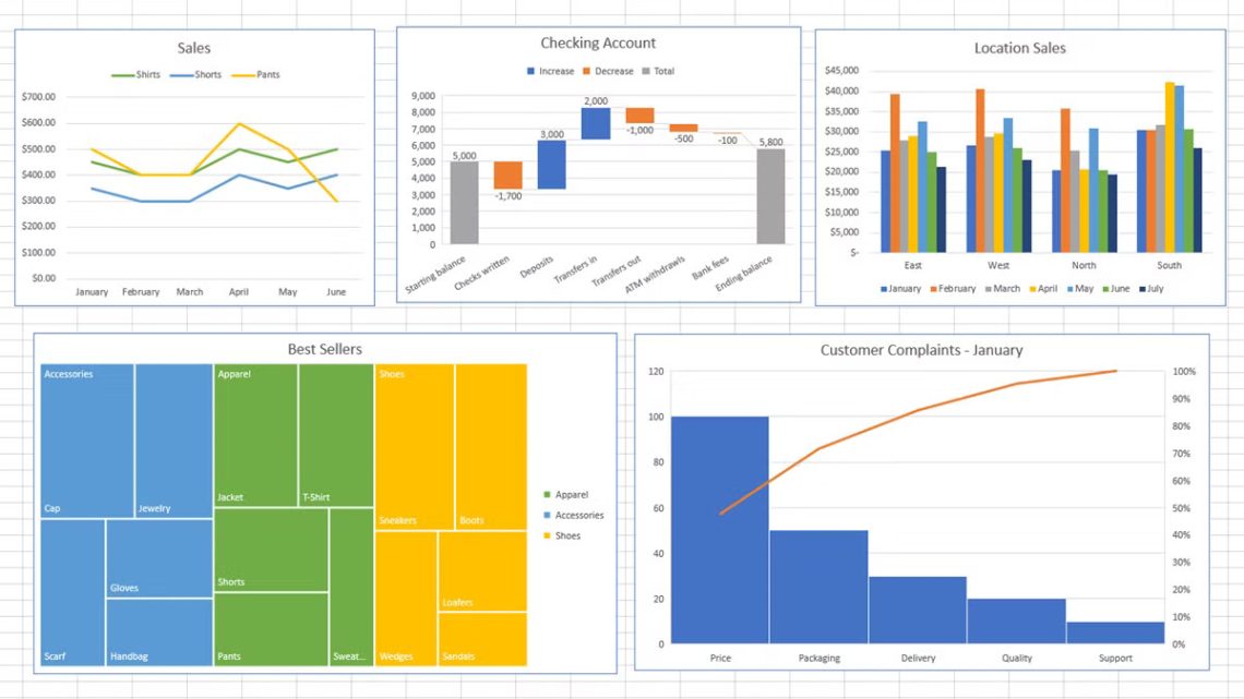
✅ Column Chart – Great for comparing values across categories (e.g., sales per region).
✅ Line Chart – Perfect for showing trends over time (e.g., monthly revenue growth).
✅ Pie Chart – Best for displaying proportions or percentages (e.g., market share breakdown).
✅ Bar Chart – Useful for comparing large datasets (e.g., employee performance).
✅ Scatter Plot – Ideal for showing relationships between two variables (e.g., sales vs. advertising spend).
✅ Combo Chart – A mix of different chart types (e.g., revenue as a bar, profit as a line).
📌 Pro Tip: Avoid pie charts when comparing too many categories—use bar charts instead for better clarity.
2️⃣ Creating a Basic Chart in Excel
Follow these steps to create a simple yet effective chart:
Step 1: Select Your Data
Highlight the data range you want to visualize. For example, if you’re tracking monthly sales, select:
| Month | Sales ($) |
|---|---|
| January | 10,000 |
| February | 12,500 |
| March | 15,000 |
| April | 14,500 |
| May | 16,800 |
Step 2: Insert a Chart
-
Click on the Insert tab.
-
Choose a chart type under the Charts section.
-
Select a chart (e.g., Line Chart for sales trends).
-
Click OK—your chart will appear in your Excel sheet!
3️⃣ Enhancing Your Charts for Maximum Impact
Now that you have a basic chart, let’s make it visually appealing!
📌 Step 1: Customize the Chart Title
Click on the default title and enter something more descriptive, e.g., “Monthly Sales Performance (2024)”.
📌 Step 2: Add Data Labels
-
Click on the chart.
-
Go to Chart Elements (the + icon).
-
Check Data Labels to display values directly on the chart.
📌 Step 3: Adjust Axis Labels
-
Click on the horizontal or vertical axis.
-
Right-click and choose Format Axis.
-
Customize the labels to be more readable (e.g., changing date formats).
📌 Step 4: Change Chart Colors & Styles
-
Click on your chart.
-
Go to the Chart Design tab.
-
Select a predefined chart style or manually change colors to match your brand.
🎨 Pro Tip: Use contrasting colors to highlight key data points—this improves readability.
4️⃣ Advanced Charting Techniques
📊 Creating a Combo Chart (Dual-Axis Chart)
If you want to compare two different data sets, such as revenue and profit, a combo chart works best.
-
Select your data (e.g., Sales & Profit).
-
Go to Insert > Combo Chart > Custom Combo Chart.
-
Set one dataset as a Column Chart and the other as a Line Chart.
-
Enable a Secondary Axis for better comparison.
📌 Best Use Case: Comparing revenue growth (bars) with profit margins (line).
📊 Creating a Dynamic Chart with Drop-Down Filters
Want to make your chart interactive? Add a drop-down filter to let users choose different categories.
-
Create a list of values in a separate column (e.g., Product Categories).
-
Use the Data Validation feature to create a drop-down list.
-
Use the INDEX/MATCH or INDIRECT formulas to dynamically update your chart based on the selected category.
🚀 Pro Tip: This is great for creating interactive dashboards in Excel!
5️⃣ Exporting & Sharing Your Charts
Once your chart is ready, you may need to share it in presentations, reports, or emails.
🖼️ Exporting as an Image
-
Click on the chart.
-
Right-click and select Save as Picture.
-
Choose a format (PNG, JPG) and save it.
📂 Copying to PowerPoint or Word
-
Select the chart and press Ctrl + C.
-
Open PowerPoint or Word and press Ctrl + V.
-
Resize and adjust as needed.
📝 Pro Tip: Use the Paste Special option to embed the chart with Excel data for future updates.
Conclusion
Excel is a powerful tool for data visualization, allowing you to create stunning charts and graphs that turn complex numbers into actionable insights. Whether you’re presenting sales data, financial reports, or survey results, using the right chart type, colors, and formatting can make your data more engaging and persuasive.
💡 Need help designing custom Excel charts for your business or project? Let’s connect! We provide tailored Excel solutions and expert consultations to enhance your workflow.